Goal of this experiment is to see if the SRM.xls "ends" workaround discovered with the "two" grain motor will work for a one grain motor. This eliminates the variable of the different grain lengths and focuses just on the "ends workaround."

The standard use of SRM.xls has the multiple grains (N) the same size/length as each other. It also has all the grain ends inhibited (Ends=0) or all ends not inhibited (Ends=1). However the multigrain motors have grains that sometimes differ in length. As in this motor one end is inhibited and the other is not.
It is hoped that the sim results of the SRM.xls thrust curve vs time can be made to correlate with static test thrust curve vs time results. This would preferably be by adjusting input rather than the more complicated approach of changing the internal calculations within SRM.xls

The motor was constructed as per the image above. The red areas shows the non-inhibited surfaces along with the ignitor.
The motor was then ignited on a static test stand to measure thrust. This is a spring weight scale. The static burn is videotaped and the thrust over time is plotted by analyzing each frame for thrust. The video captures 30 frames per second.
The sim results are obtained by entering the chamber and grain data into the Excel file and solving for output.
Once these graphs are available they are roughly compared for maximum thrust, burn time, and if the thrust curve is neutral, progressive, or regressive.
Any obvious differences in the sim file are addressed by changing input into the SRM.xls file.
Of course the input changes need to reflect reality so the focus is changes that reflect the non-standard construction of these grains.

Each graph below shows the static results from two motors (motor #89 in green and #97 in red) against the sim results (in black). In each succesive graph the sim is changed by changing the "ends" input (ends = 1, 0, and 0.5)


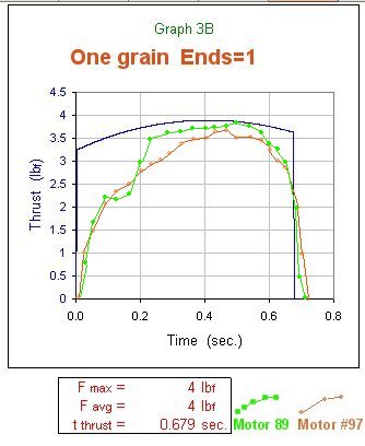
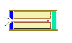
The graph above has the sim with ends=1 so SRM calculates both ends burning. This gives an expected fairly neutral burn. The two statics though are somewhat progressive. Not surprising since one end is inhibited. (See motor image above, red areas represent unhibited surfaces at ignition.


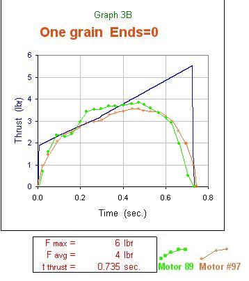
Above is the sim with ends=0 meaning that both ends are calculated as inhibited.
Like the "two" (1.5) grain motor (my standard D16 motor) the second half of the static burn is not as progressive as the sim.
Again this makes sense since the static motors have one end per grain exposed.
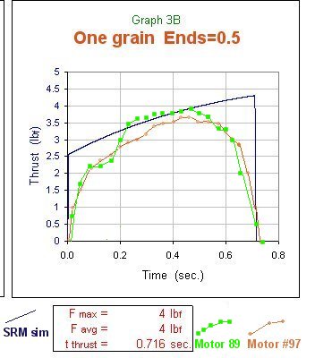
So once again to compensate in the sim input we enter ends=0.5
This will calculate that one end burns and the other is inhibited.
Now.. does the adjusted sim reflect reality?
See graph image below:

For the three sims above the third sim with the 0.5 ends workaround seems to best portray the semi-progressive curve of the burn. The sim start up and tail off are overly "optimistic". Motors with longer burn times (IE larger motors with deeper web thickness) would probably be better for this experiment. One could focus on a longer time period of full burn pressure change over time. Even my multigrain motors seem to be better for this though they do not have a longer burn time.

A second bit of information from this experiment is the reproducibility between two motors. The graphs of motors #89 and #97 look pretty darn good (darn close) to me.
(how's that for statistical analysis? ;-)



To further test this process one could try a variety of motor/grain configurations to see if these workarounds keep the predictive value of SRM.
See the results for:
The one grain motor ...That link is this page
The standard "two" grain motor
The two grain booster motor
The two full grain motor
The three grain motor


Another question is the reproducibility of these small motors. Too much variation in performance would make all this "fine tuning" of the sims a mute point. The one grain page listed above includes 2 static motors side by side.
Click Here to see a preliminary comparison of four standard "two" grain motor statics.





Back to Drysophila-Sorbitol Project Main Page